Beginnings

When I was younger, I got my hands on a copy of The Fractal Nature of Geometry by Benoit Mandelbrot. To my young mind, this revealed a fascinating new world of math with algorithms that promised to shape mountains and trees and, best of all, seemed to suggest a hidden landscape of complexity and seeming irregularity that lurked just underneath the simple and familiar mathematics that I knew.

Still etched in my mind, long after reading it, were images and names like the Sierpinski triangle, Peano curves, Hilbert curves, Julia sets, etc. As I grew older, my interests fanned out and the demands of daily life left me less time and energy to spend on these interests. So, while these things certainly still intrigued me, they came to mind less and less.

So I was pleasantly surprised a couple of months ago when my team began discussing the possibility of storing geospatial data in Microsoft’s Cosmos database and I read through the documentation to find that the implementation encoded geospatial coordinates as a Hilbert curve distance so that this distance could be used to create a searchable index. The idea made perfect sense to me but at the time, I had no idea how to map a distance to a Hilbert curve (or vice versa). The concept was interesting but, once again, life stepped in and my focus was driven elsewhere.

In mid-January, though, as I was working through a test case and wanted to generate a set of randomly-distributed coordinates, I started thinking about how a single random number between zero and one might be used to generate each of the coordinate pairs that I wanted if I treated the number as a Hilbert distance. While I went on to address this test in a different way, I went home thinking about mapping a distance to coordinates.

Looking For Direction

So, early on, I visited the Hilbert curve Wikipedia page, which featured an image of a three-dimensional Hilbert curve, an image labelled “production rules”, and C language source code for an algorithm to map between a distance value and a pair of coordinates on a Hilbert curve (and back again). The algorithm would have been very helpful if all I wanted to do was to implement the mapping – I could just port the code and walk away – but, by now, I was eager to pull the lid off of the Hilbert curve and take a look at what “made it work”.

By now, the three dimensional Hilbert curve begged the question, “how do I map between a distance and three coordinates, or five, or more?” Further, I wondered what would a three-dimensional slice of an N-dimensional Hilbert curve even look like? Why did the second order (or second degree as I fell into the habit of calling it) of a two-dimensional Hilbert curve turn head “right” at the onset rather than “up” like its first order ancestor? Yes, the “production rules” image said that this was the case but my question wasn’t about “what” the curve did – I was interested in “why?”

The most valuable clue that I found on the entire page turned out to be the statement that “Hilbert curves in higher dimensions are an instance of a generalization of Gray codes…” (somehow the statement that ” there are several possible generalizations of Hilbert curves to higher dimensions” and the associated footnote link to the paper entitled On Multidimensional Curves With Hilbert Property escaped my notice) It took a bit of exploration on my part before the importance of this statement really sank in.

Happily, for me, none of my searches turned up anything more helpful than this regarding the fundamental algorithm and I was left with this set of questions steadily growing roots in the back of my mind. I say “happily” because there is much greater satisfaction (and understanding) to be gained for an answer that is hard won versus one that is simply handed to me faît accomplis.

Finding My Way

So, without further guidance, I began to pick apart the Hilbert curve on my own. It didn’t take long to apply the production rules and demonstrate that, yes, if you follow the rules given, you end up with a nice two-dimensional Hilbert curve of any arbitrary order you want. I hacked together a method in Java that (or maybe I was working from someone else’s code that I had stumbled across) that selected the second order curve to insert based on the last segment that the algorithm had generated and the next segment in the ancestor curve. The algorithm looked essentially like this:

    Orientation2D[] expand2d(Orientation2D previous, Orientation2D next) {

        Orientation2D[] StepUp =    { Right, Up, Left };
        Orientation2D[] StepRight = { Up, Right, Down };
        Orientation2D[] StepDown =  { Left, Down, Right };
        Orientation2D[] StepLeft =  { Down, Left, Up, };

        if (previous == Up && next == Up)
            return StepUp;

        if (previous == Right && next == Up)
            return StepUp;

        if (previous == Up && next == Left)
            return StepUp;


        if (previous == Down && next == Down)
            return StepDown;

        if (previous == Down && next == Right)
            return StepDown;

        if (previous == Left && next == Down)
            return StepDown;


        if (previous == Right && next == Right)
            return StepRight;

        if (previous == Up && next == Right)
            return StepRight;

        if (previous == Right && next == Down)
            return StepRight;


        if (previous == Left && next == Left)
            return StepLeft;

        if (previous == Down && next == Left)
            return StepLeft;

        if (previous == Left && next == Up)
            return StepLeft;


        throw new RuntimeException();
    }

It wasn’t pretty but it wasn’t intended to be – all I needed at this point was a generator for an arbitrary curve so that I could look more closely at the results and try to extract a pattern. The interpreter for the resulting output simply incremented X when it encountered a Right instruction, decremented X when it encountered a Left instruction, incremented Y when it encountered an Up instruction, and decremented Y when it encountered a Down instruction.

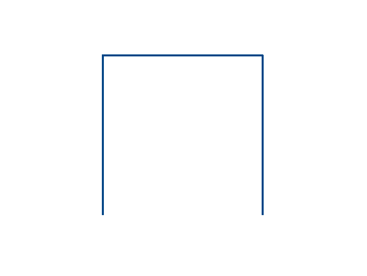
One of the first things that I noticed about the output was that the first order curve had three steps such that, if it began at (0, 0), it would end at (1,0) and that the net effect of the curve was to advance to the right by one (when looking exclusively at the start point and end point).

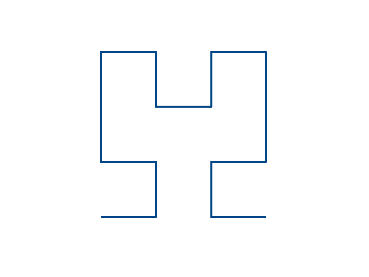
Meanwhile, the second order curve had fifteen steps such that, if it began at (0, 0), it would end at (3, 0) and the third order curve had sixty-three steps such that, if it began at (0,0), it would end at (7, 0). The clear linkage between the degree, the extents of the curve in the 2d coordinate space, and the length of the curve wasn’t lost on me but I still didn’t quite get what I was looking at.

I took some time to attempt the same decomposition for the construction of a 3d Hilbert curve but it didn’t take long before I realized that this was going to take a lot of effort and that I probably wouldn’t get any closer. Instead, I change gear and looked closely at a second order 3d Hilbert curve so that I could decompose it into a set of Up, Down, Left, Right, Away, and Toward instructions. I then generated a first and second order Hilbert curve and looked at the results.

Interestingly, the resulting set of instructions and extents showed a similar pattern to the 2d curve. The first order curve in two dimensions starting at (0,0) traveled up to (0, 1), then right to (1, 1), then finally traveled down to (0, 1) so that it visited all four vertices of a unit square. The first order curve in three dimensions starting at (0, 0, 0) traveled away to (0, 0, 1), then up to (0, 1, 1), then toward to (0, 1, 0), then right to (1, 1, 0), then away to (1, 1, 1), then down to (1, 0, 1), and finally toward to (1, 0, 0) so that the net movement was, again, one step to the right but only after visiting all eight vertices of a unit cube.

It began to sink in that, at each order, the resulting 2d Hilbert curve visited every vertex of every unit square within whatever area it covered. Similarly, the 3d Hilbert curve visited every vertex of every unit cube of whatever volume it covered. Maybe this doesn’t really seem like headline stuff – after all, the Hilbert curve is categorized as a “space filling curve” so it seems pretty natural that this is exactly what it would do. The thing that changed here, however, was my perspective on the movements required to accomplish this.

Black And White (But Gray All Over)

I finally turned to look again at the first order curve again and I finally noticed what the coordinates were telling me. If I took the first order 2d curve and treated the coordinates as a binary number, the sequence was simply:

00
01
11
10

Meanwhile, if I took the first order 3d curve and treated its coordinates as a binary number, the sequence became:

000
001
011
010
110
111
101
100

If you’re at all familiar with Gray code, you will probably recognize this sequence (and if you’re not, the Gray code Wikipedia page can tell you all sorts of things about it). This observation is central to the mechanism behind the generation of a Hilbert curve because each transition from one vertex to another in a Hilbert curve in any dimension travels along an edge – never along a diagonal. Saying this another way: along a Hilbert curve, moving from one vertex to the next always involves changing the value of only one coordinate (e.g. X or Y may change but never X and Y). This is exactly what a Gray code achieves.

Gray codes have been used in software and hardware because they possess this property: the transition from any Gray code value to the next Gray code value involves a change to the value of a exactly one bit. This is valuable in communication and positioning because the hardware or software can easily test for a change to two or more bits between adjacent values and report an error (e.g. to report an error and halt the movement of a robotic arm because the positioning sensor has become dirty and, therefore, unreliable).

Another interesting property of a Gray code is that any permutation of a Gray code is also a Gray code. That is, if we label the bits of our Gray code A, B, and C, the sequence in ABC (000, 001, 011, 010, 110, 111, 101, 100) can be remapped to BCA as (000, 010, 110, 100, 101, 111, 011, 001) but this sequence remains a Gray code. Our fist sequence in ABC corresponds to a Hilbert curve that originates at (0, 0, 0) and terminates at (1, 0, 0) while our second corresponds to a Hilbert curve that originates at (0, 0, 0) and terminates at (0, 0, 1). In effect, we can act as though we have a set of basis vectors that A, B, and C to X, Y, and Z and we can use this to orient our first order Hilbert curve so that it progresses up, right, or away.

So the Wikipedia article on the Hilbert curve really sort of buries the headline with the assertion that “Hilbert curves in higher dimensions are an instance of a generalization of Gray codes…” because any first order Hilbert curve is nothing more than a Gray code.

Turning To Progress In A New Direction

So, this is an important milestone – we can use this to construct a first order Hilbert curve in any number of dimensions. Moreover, we can find the set of coordinates for any vertex on this first order Hilbert from a simple distance value by converting that distance value to its corresponding Gray code value. In many languages (e.g. C, C++, Java, C#, etc.) we accomplish this easily with the statement:

long grayCode = value ^ (value >> 1);

Thinking about the process of generating a Hilbert curve, then, it seems that we can generate our second order Hilbert curve by simply replacing a segment along its path with the set of segments whose beginning and end map to that segment’s beginning and end. To illustrate this idea, we can look at the 2d Hilbert curve

The first order Hilbert curve is generated from a two bit Gray code:

AB   # (X, Y)
-------------
00   # (0, 0)
01   # (0, 1)
11   # (1, 1)
10   # (1, 0)

This curve moves from the left to the right but it does so by first moving up from (0, 0) to (0, 1). We can find the appropriate variation of the first order 2d curve by simply exchanging the order of our A and B bits (or rotating the bits in AB):

BA    # (X, Y)
--------------
00    # (0, 0)
10    # (1, 0)
11    # (1, 1)
01    # (0, 1)

Another way to think about this (though not a particularly efficient way to calculate it) is to imagine that we have our simple set of bits that encode our Gray code values (e.g. AB) and that we have a matrix that maps these AB bits onto our X, Y coordinate values. The matrix:

gives us A, B as X, Y while the matrix:

gives us B, A as X, Y.

So, we can construct our progress from (0, 0) in the second order 2d Hilbert curve by changing the mapping of (A, B) to (X, Y) so that X=B and Y=A in the (0, 0) quadrant. Then observation shows that the next two sections of the second order Hilbert curve are simply repeats of the first order curve but at different starting points so, here the mapping is once again X=A and Y=B in the (0, 2) and (2, 2) quadrants.

Reflecting On The Results

Still, we’re not quite there yet because when we reach the final leg of the first order Hilbert curve ancestor, and descend from (1, 1) to (1, 0), we have two problems.

Our first problem is that this section of the curve starts at (3, 1) and ends at (3, 0) so it would require a version of our first order Hilbert curve that starts at (1, 1) and ends at (1, 0). But there is simply no permutation of our A and B bits that will start at 11 and end at 10.

Our second problem is that, in this section of the curve, our X coordinate value must decrease during its movement from (1, 1) to (1, 0) in order to reach two of the four remaining unit square vertices at (2, 1) and (2, 0). Once again, there is simply no permutation of our A and B bits that will accomplish this for us. So, what is going on here?

Well, if you’re geometrically-minded, you’ve probably intuited that there is a left-right mirror symmetry to the second order Hilbert curve in 2d (in fact, it turns out that symmetry is an essential feature of Hilbert curves of all dimensions and of all orders). Once we reach the midpoint along our Hilbert curve, we’re actually travelling backwards over a reflection of the original curve.

A particularly convoluted (but very precise) way of looking at this is to say that, starting at the midpoint of our Hilbert curve, we begin to compute points based on a decreasing distance along a left-right mirror image of the first half of our Hilbert curve. Here is the convoluted (but precise) part:

If we were simply travelling backwards, we would be retracing the same set of coordinates. Since we are, instead, traversing a left-right mirror image of the first half of the Hilbert curve, we move right when would would move left. As a result, we continue to move right until we reach X=3 and then we progress down. Now, from (3, 1) to (3, 0), we traverse the mirror image of our first order Hilbert curve from the first quadrant by moving from (1, 1), to (0, 1), to (0, 0), and finally to (1, 0).

Connecting The Dots

So, at this point, we have all of the elements required to construct an algorithm to compute a point along an arbitrary dimension, arbitrary order Hilbert curve and the trick is just putting them together. Moreover, we actually have everything we need to convert from a set of coordinates back to a distance value. The only thing that remains is to put them together to give us the result that we want.

As I’m sure you’d have already guessed by now, I’ve already created an implementation of the code to do this and I’ve posted it in my Github repository as HilbertCurveExample. It feels like there are probably a few loose ends to tie up so I may return with a follow-up post.

Wikipedia

In case you can’t tell, I rely heavily on Wikipedia as a fantastic (and, I believe, seriously undervalued) resource for a lot of my resource. I make it a point to donate and I would like to encourage anyone reading this to donate to Wikipedia too